Elasticsearch 很快。快到很多人把它拿來當資料庫用,然後發現資料不見了。因為 ES 不是資料庫——它是搜尋引擎,擅長全文檢索跟聚合分析,但不保證 ACID。
先講結論
ES 的三個核心你一定要搞懂:Mapping 決定你怎麼查、Shard 決定你能撐多大、ILM 決定你花多少錢。Mapping 一旦建了很難改,Shard 太多太少都是災難,ILM 不設就等著磁碟爆炸。把這三件事做對,ES 會是你的好幫手;做錯的話,它會是你的噩夢。
Mapping:一開始就要想好
Mapping 就是 ES 的 schema。最重要的決定是字串欄位要用 text 還是 keyword:
text:會被分詞,用在全文搜尋(「搜尋包含某個詞的文件」)keyword:不分詞,用在精確匹配跟聚合(「篩選 status = active」)
PUT /products
{
  "mappings": {
    "properties": {
      "name": { "type": "text", "analyzer": "standard" },
      "sku":  { "type": "keyword" },
      "price": { "type": "double" },
      "created_at": { "type": "date" }
    }
  }
}
不要依賴 dynamic mapping。 ES 會自動猜你的欄位類型,但它猜的常常不是你要的。第一筆資料進來的時候 ES 把一個欄位設成 text,後來你想拿它做聚合才發現需要 keyword——但 mapping 改不了,只能 reindex 整個 index。
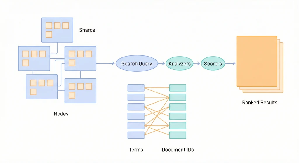
Shard 策略:太多太少都不行
每個 index 由多個 shard 組成。Shard 太多,集群管理開銷大、記憶體被吃光。Shard 太少,單一 shard 太大,rebuild 跟搬移都很慢。
經驗法則:單一 shard 控制在 20-50GB。
規劃步驟:
- 估算一年的資料量
- 除以目標 shard 大小 → 得到 shard 數量
- 用時間滾動 index(例如每月一個 index),配合 ILM 自動管理
大量小 shard 是新手最常犯的錯——每天一個 index 但每天只有幾 MB 資料,一年下來有三百多個幾乎空的 index,每個還占著 cluster state 的記憶體。
Query DSL:Filter 比 Query 重要
ES 的查詢分兩種:query(計算相關性分數)跟 filter(純過濾,不計分)。Filter 可以被快取,效能好很多。
GET /products/_search
{
  "query": {
    "bool": {
      "must": [
        { "match": { "name": "wireless" } }
      ],
      "filter": [
        { "term": { "status": "active" } }
      ]
    }
  }
}原則很簡單:能用 filter 的就不要用 query。status = active 不需要計算相關性,放在 filter 裡就好。只有真正需要做全文搜尋、排名的欄位才放在 must 裡。
ILM:不做就等著磁碟爆炸
ILM(Index Lifecycle Management)控制 index 在不同階段的行為:
- Hot:高頻寫入,用 SSD
- Warm:讀取為主,可以用便宜的磁碟
- Cold:低頻查詢,壓縮儲存
- Delete:過期刪除
如果你不設 ILM,index 就會無限長大,直到磁碟滿了、cluster 變 red、然後你在半夜被叫起來刪資料。
寫入路由固定指向 Hot 節點。ILM policy 設定 rollover 條件(例如 index 超過 50GB 或 30 天就滾動)。過期 index 自動刪除前確認合規需求。
監控:這些指標必看
ES cluster 的健康狀態只有三種顏色:green(全部正常)、yellow(有 replica 沒分配)、red(有 primary shard 沒分配)。
除了 cluster health,你至少要監控:
- JVM heap 使用率(不要超過 75%)
- GC 時間跟頻率(頻繁 GC 是記憶體不夠的訊號)
- Search latency(p95 / p99)
- Segment merge 時間
JVM heap 配置的經驗法則:不超過主機記憶體的 50%,最多不超過 32GB(超過 32GB 會失去 compressed oops)。剩下的記憶體留給 OS filesystem cache——ES 的 segment 檔案依賴 OS cache 來加速讀取。
延伸閱讀
- Elasticsearch Official Docs
- ILM Best Practices
- Search Performance Tuning
Elasticsearch 最常見的死因不是流量太大,而是沒人管理 index 生命週期。它就靜靜地長大,直到有一天磁碟滿了、cluster red 了、然後所有人才驚覺:原來搜尋引擎也需要做運維。