Google Maps 怎麼算出最短路線?Dijkstra + A*。網路路由器怎麼決定封包往哪走?Dijkstra。金融系統怎麼偵測套利機會?Bellman-Ford 找負環。圖演算法不是學術題目,它藏在你每天用的工具裡。
先講結論
| 你想做什麼 | 用什麼 | 時間複雜度 |
|---|---|---|
| 單源最短路徑(無負權) | Dijkstra | O((V+E) log V) |
| 單源最短路徑(有負權) | Bellman-Ford | O(V×E) |
| 所有點對最短路徑 | Floyd-Warshall | O(V³) |
| 點對點(有啟發函數) | A* | O(E) 最佳 |
沒有負權重 → Dijkstra。有負權重 → Bellman-Ford。要算所有配對 → Floyd-Warshall。地圖導航 → A*。就這麼簡單。
Dijkstra:貪心找最短路
核心思想:每次從「還沒確定」的節點中,挑距離最小的。一旦挑中,它的最短距離就確定了(因為沒有負權重,後面不可能更短)。
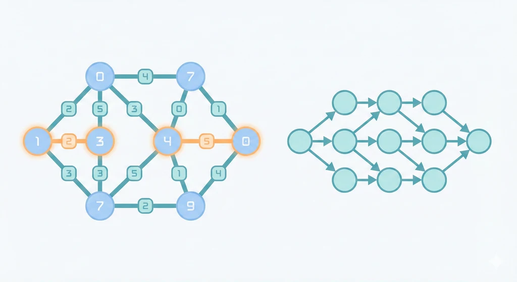
從節點 1 出發:
1. dist = [0, ∞, ∞, ∞]
2. 更新 1 的鄰居:dist = [0, 4, 2, ∞]
3. 選最小的 3(dist=2)→ 確定
4. 更新 3 的鄰居:dist = [0, 4, 2, 5]
5. 選最小的 2(dist=4)→ 確定
6. 最後 4(dist=5)→ 確定
用 Priority Queue 實作:
int[] dijkstra(Graph g, int source) {
    int[] dist = new int[V];
    Arrays.fill(dist, INF);
    dist[source] = 0;

    PriorityQueue<int[]> pq = new PriorityQueue<>((a,b) -> a[0]-b[0]);
    pq.offer(new int[]{0, source});

    while (!pq.isEmpty()) {
        int[] curr = pq.poll();
        int d = curr[0], u = curr[1];
        if (d > dist[u]) continue;  // 已有更短路徑

        for (Edge e : neighbors(u)) {
            int newDist = dist[u] + e.weight;
            if (newDist < dist[e.to]) {
                dist[e.to] = newDist;
                pq.offer(new int[]{newDist, e.to});
            }
        }
    }
    return dist;
}
致命限制:不能有負權重邊。 為什麼?因為 Dijkstra 的貪心假設是「確定的節點不會再被更新」。負權重會打破這個假設。
Bellman-Ford:暴力但萬用
對所有邊做 V-1 次鬆弛。暴力?是的。但它能處理負權重,還能偵測負環。
for (int i = 0; i < V - 1; i++) {
    for (每條邊 (u, v, w)) {
        if (dist[u] + w < dist[v]) {
            dist[v] = dist[u] + w;
        }
    }
}

// 第 V 次還能更新 = 有負環
for (每條邊 (u, v, w)) {
    if (dist[u] + w < dist[v]) return "有負環!";
}
工程場景:外匯市場的套利偵測。把幣別當節點、匯率取 log 當邊權重,如果存在負環,就表示有套利機會(換一圈回來錢變多了)。
Floyd-Warshall:所有配對
三層迴圈,DP 思維:「從 i 到 j,允許經過節點 0~k 的最短路徑是多少?」
for (int k = 0; k < V; k++)
    for (int i = 0; i < V; i++)
        for (int j = 0; j < V; j++)
            dist[i][j] = min(dist[i][j], dist[i][k] + dist[k][j]);
O(V³) 聽起來很慢,但如果你需要所有配對的最短路徑,它是最簡單的選擇。而且只有三行核心程式碼,debug 的時候非常舒服。
A*:比 Dijkstra 更聰明
Dijkstra 像無頭蒼蠅,往所有方向擴展。A* 多了一個啟發函數 h(n),估計從 n 到終點的距離,讓搜尋方向朝目標前進。
f(n) = g(n) + h(n)
g(n) = 起點到 n 的實際距離
h(n) = n 到終點的估計距離
常用的啟發函數:
- 曼哈頓距離(|x1-x2| + |y1-y2|):網格地圖,只能上下左右
- 歐幾里得距離:任意方向移動
- 切比雪夫距離(max(|Δx|, |Δy|)):含對角線移動
Google Maps 用的就是 A* 的變體。地圖資料是一張巨大的加權圖(路口=節點、道路=邊),用直線距離當啟發函數,避免向反方向搜尋。實際的生產系統會再加上 Contraction Hierarchies 等預處理,讓查詢從數秒降到毫秒。
拓撲排序和其他進階圖論主題請看 圖演算法(下):拓撲排序與工程應用。
Dijkstra 在 1956 年用 20 分鐘想出了這個演算法。我用了 20 分鐘理解它,然後又用了 2 小時 debug 我的 Priority Queue 實作。